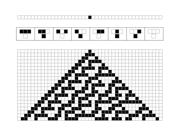
SO, why’s an urban fantasy author digging into the guts of Mathematica trying to reverse-engineer how Stephen Wolfram drew the diagrams of cellular automata in his book A New Kind of Science? Well, one of my favorite characters to write about is the precocious teenage weretiger Cinnamon Frost, who at first glance was a dirty little street cat until she blossomed into a mathematical genius when watered with just the right amount of motherly love. My training as a writer was in hard science fiction, so even if I’m writing about implausible fictions like teenage weretigers, I want the things that are real – like the mathematics she develops – to be right. So I’m working on a new kind of math behind the discoveries of my little fictional genius, but I’m not the youngest winner of the Hilbert Prize, so I need tools to help simulate her thought process.
And my thought process relies on visualizations, so I thought, hey, why don’t I build on whatever Stephen Wolfram did in his groundbreaking tome A New Kind of Science, which is filled to its horse-choking brim with handsome diagrams of cellular automata, their rules, and the pictures generated by their evolution? After all, it only took him something like ten years to write the book … how hard could it be?
Deconstructing the Code from A New Kind of Science, Chapter 2
Fortunately Stephen Wolfram provides at least some of the code that he used for creating the diagrams in A New Kind of Science. He’s got the code available for download on the book’s website, wolframscience.com, but a large subset is in the extensive endnotes for his book (which, densely printed and almost 350 pages long, could probably constitute a book in their own right). I’m going to reproduce that code here, as I assume it’s short enough to fall under fair use, and for the half-dozen functions we’ve got here any attempt to reverse-engineer it would end up just recreating essentially the same functions with slightly different names.
Cellular automata are systems that take patterns and evolve them according to simple rules. The most basic cellular automata operate on lists of bits – strings of cells which can be “on” or “off” or alternately “live” or “dead,” “true” and “false,” or just “1” and “0” – and it’s easiest to show off how they behave if you start with a long string of cells which are “off” with the very center cell being “on,” so you can easily see how a single live cell evolves. And Wolfram’s first function gives us just that, a list filled with dead cells represented by 0 with a live cell represented by 1 in its very center:
In[1]:= CenterList[n_Integer] := ReplacePart[Table[0, {n}], 1, Ceiling[n/2]]
In[2]:= CenterList[10]
Out[2]= {0, 0, 0, 0, 1, 0, 0, 0, 0, 0}
One could imagine a cellular automata which updated each cell just based on its contents, but that would be really boring as each cell would be effectively independent. So Wolfram looks at what he calls “elementary automata” which update each cell based on their neighbors. Counting the cell itself, that’s a row of three cells, and there are eight possible combinations of live and dead neighbors of three elements – and only two possible values that can be set for each new element, live or dead. Wolfram had a brain flash to list the eight possible combinations the same each way every time, so all you have are that list of eight values of “live” or “dead” – or 1’s and 0’s, and since a list of 1’s and 0’s is just a binary number, that enabled Wolfram to represent each elementary automata rule as a number:
In[3]:= ElementaryRule[num_Integer] := IntegerDigits[num, 2, 8]
In[4]:= ElementaryRule[30]
Out[4]= {0, 0, 0, 1, 1, 1, 1, 0}
Once you have that number, building code to apply the rule is easy. The input data is already a string of 1’s and 0’s, so Wolfram’s rule for updating a list of cells basically involves shifting (“rotating”) the list left and right, adding up the values of these three neighbors according to base 2 notation, and then looking up the value in the rule. Wolfram created Mathematica in part to help him research cellular automata, so the code to do this is deceptively simple…
In[5]:= CAStep[rule_List, a_List] :=
rule[[8 – (RotateLeft[a] + 2 (a + 2 RotateRight[a]))]]
… a “RotateLeft” and a “RotateRight” with some addition and multiplication to get the base 2 index into the rule. The code to apply this again and again to a list to get the history of a cellular automata over time is also simple:
In[6]:= CAEvolveList[rule_, init_List, t_Integer] :=
NestList[CAStep[rule, #] &, init, t]
Now we’re ready to create the graphics for the evolution of Wolfram’s “rule 30,” the very simple rule which shows highly complex and irregular behavior, a discovery which Wolfram calls “the single most surprising scientific discovery [he has] ever made.” Wow. Let’s spin it up for a whirl and see what we get!
In[7]:= CAGraphics[history_List] :=
Graphics[Raster[1 – Reverse[history]], AspectRatio -> Automatic]
In[8]:= Show[CAGraphics[CAEvolveList[ElementaryRule[30], CenterList[103], 50]]]
Out[8]=
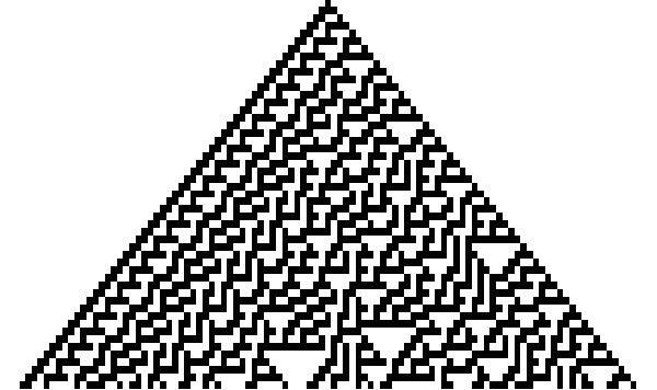
Uh – oh. The “Raster” code that Wolfram provides is the code to create the large images of cellular automata, not the sexy graphics that show the detailed evolution of the rules. And reading between the lines of Wolfram’s end notes, he started his work in FrameMaker before Mathematica was ready to be his full publishing platform, with a complex build process producing the output – so there’s no guarantee that clean simple Mathematica code even exists for some of those early diagrams.
Guess we’ll have to create our own.
Visualizing Cellular Automata in the Small
The cellular automata diagrams that Wolfram uses have boxes with thin lines, rather than just a raster image with 1’s and 0’s represented by borderless boxes. They’re particularly appealing because the lines are white between black boxes and black between white boxes, which makes the structures very easy to see. After some digging, I found that, naturally, a Mathematica function to create those box diagrams does exist, and it’s called ArrayPlot, with the Mesh option set to True:
In[9]:= ArrayPlot[Table[Mod[i + j, 2], {i, 0, 3}, {j, 0, 3}], Mesh -> True]
Out[9]=
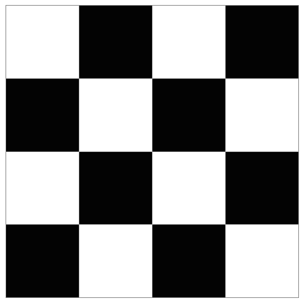
While we could just use ArrayPlot, it’ s important when developing software to encapsulate our knowledge as much as possible, so we’ll create a function CAGridGraphics (following the way Wolfram named his functions) that encapsulates the knowledge of turning the Mesh option to True. If later we decide there’s a better representation, we can just update CAMeshGraphics, rather than hunting down every use of ArrayPlot. This function gives us this:
In[10]:= CAMeshGraphics[matrix_List] :=
ArrayPlot[matrix, Mesh -> True, ImageSize -> Large]In[11]:= CAMeshGraphics[{CenterList[10], CenterList[10]}]
Out[11]=

Now, Wolfram has these great diagrams to help visualize cellular automata rules which show the neighbors up top and the output value at bottom, with a space between them. The GraphicsGrid does what we want here, except it by its nature resizes all the graphics to fill each available box. I’m sure there’s a clever way to do this, but I don’t know Mathematica well enough to find it, so I’m going to go back on what I just said earlier, break out the options on ArrayPlot, and tell the boxes to be the size I want:
In[20]:= CATransitionGraphics[rule_List] :=
GraphicsGrid[
Transpose[{Map[
ArrayPlot[{#}, Mesh -> True, ImageSize -> {20 Length[#], 20}] &, rule]}]]
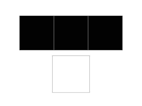
That works reasonably well; here’ s an example rule, where three live neighbors in a row kills the center cell :
In[21]:= CATransitionGraphics[{{1, 1, 1}, {0}}]
Out[21]=
Now we need the pattern of digits that Wolfram uses to represent his neighbor patterns. Looking at the diagrams and sfter some digging in the code, it seems like these digits are simply listed in reverse counting order – that is, for 3 cells, we count down from 2^3 – 1 to 0, represented as binary digits.
In[22]:= CANeighborPattern[num_Integer] :=
Table[IntegerDigits[i, 2, num], {i, 2^num – 1, 0, -1}]In[23]:= CANeighborPattern[3]
Out[23]= {{1, 1, 1}, {1, 1, 0}, {1, 0, 1}, {1, 0, 0}, {0, 1, 1}, {0, 1, 0}, {0, 0,
1}, {0, 0, 0}}
Stay with me – that only gets us the first row of the CATransitionGraphics; to get the next row, we need to apply a rule to that pattern and take the center cell:
In[24]:= CARuleCenterElement[rule_List, pattern_List] :=
CAStep[rule, pattern][[Floor[Length[pattern]/2]]]
In[25]:= CARuleCenterElement[ElementaryRule[30], {0, 1, 0}]
Out[25]= 1
With all this, we can now generate the pattern of 1′ s and 0′ s that represent the transitions for a single rule:
In[26]:= CARulePattern[rule_List] :=
Map[{#, {CARuleCenterElement[rule, #]}} &, CANeighborPattern[3]]In[27]:= CARulePattern[ElementaryRule[30]]
Out[27]= {{{1, 1, 1}, {0}}, {{1, 1, 0}, {1}}, {{1, 0, 1}, {0}}, {{1, 0, 0}, {1}}, {{0,
1, 1}, {0}}, {{0, 1, 0}, {1}}, {{0, 0, 1}, {1}}, {{0, 0, 0}, {0}}}
Now we can turn it into graphics, putting it into another GraphicsGrid, this time with a Frame.
In[28]:= CARuleGraphics[rule_List] :=
GraphicsGrid[{Map[CATransitionGraphics[#] &, CARulePattern[rule]]},
Frame -> All]In[29]:= CARuleGraphics[ElementaryRule[30]]
Out[29]=

At last! We’ ve got the beautiful transition diagrams that Wolfram has in his book. And we want to apply it to a row with a single cell:
In[30]:= CAMeshGraphics[{CenterList[43]}]
Out[30]=
![]()
What does that look like? Well, we once again take our CAEvolveList function from before, but rather than formatting it with Raster, we format it with our CAMeshGraphics:
In[31]:= CAMeshGraphics[CAEvolveList[ElementaryRule[30], CenterList[43], 20]]
Out[31]=
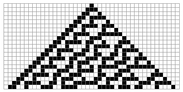
And now we’ ve got all the parts of the graphics which appear in the initial diagram of this page. Just to work it out a bit further, let’s write a single function to put all the graphics together, and try it out on rule 110, the rule which Wolfram discovered could effectively simulate any possible program, making it effectively a universal computer:
In[22]:= CAApplicationGraphics[rule_Integer, size_Integer] := Column[
{CAMeshGraphics[{CenterList[size]}],
CARuleGraphics[ElementaryRule[rule]],
CAMeshGraphics[
CAEvolveList[ElementaryRule[rule], CenterList[size],
Floor[size/2] – 1]]},
Center]In[23]:= CAApplicationGraphics[110, 43]
Out[23]=
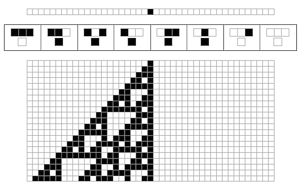
It doesn’ t come out quite the way it did in Photoshop, but we’ re getting close. Further learning of the rules of Mathematica graphics will probably help me, but that’s neither here nor there. We’ve got a set of tools for displaying diagrams, which we can craft into what we need.
Which happens to be a non-standard number system unfolding itself into hyperbolic space, God help me.
Wish me luck.
-the Centaur
P.S. While I’ m going to do a standard blogpost on this, I’ m also going to try creating a Mathematica Computable Document Format (.cdf) for your perusal. Wish me luck again – it’s my first one of these things.
P.P.S. I think it’ s worthwhile to point out that while the tools I just built help visualize the application of a rule in the small …
In[24]:= CAApplicationGraphics[105, 53]
Out[24]=
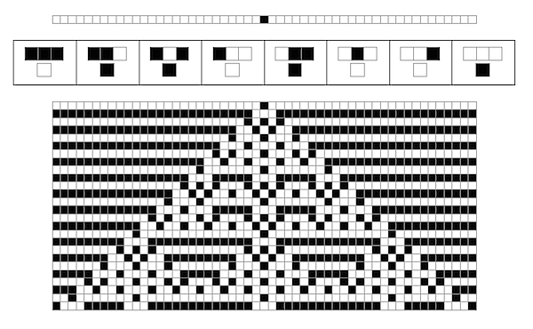
… the tools Wolfram built help visualize rules in the very, very large:
In[25]:= Show[CAGraphics[CAEvolveList[ElementaryRule[105], CenterList[10003], 5000]]]
Out[25]=
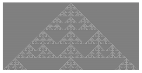
That’s 10,000 times bigger – 100 times bigger in each direction – and Mathematica executes and displays it flawlessly.